library(terra)
library(tidyterra)
library(ggplot2)
library(here)
library(foreach)
library(sf)terra package quirks
R
Spatial
In this post, I document some quirks of the terra package that may not be intuitive to new users.
terra package quirks
Overview
The issue we have encountered using the terra package is that the rasterization of vector polygons is not always intuitive, leading to some unexpected results.
Two common issues that I would like to address in this post:
terra::rasterizemisses very small polygonsterra:cropunexpectedly misses raster cells when cropping with a vector layer extent withmask = true
Setup
terra::rasterize misses very small polygons
Example
Here, providing a demonstration of the difference in output of terra::rasterize depending on whether or not touches = T. The default is touches = F, which can leave out parts or even entire polygons when rasterizing. We are using the Key Biodiversity Areas (KBAs) shapefiles in this example, which vary significantly in area and shape. The raster resolution is set at 400m.
Important
rasterize all KBAs with defaults
rasterize can miss polygons that are smaller than the cell:
# loading Key Biodiversity Areas
kba_vect <- vect(here(
  "posts/terra_package_quirks/key_biodiversity_areas/kba.20240514080519.shp"
)) |>
  project("epsg:3005") # reproject to BC Albers
ext_rast <- rast(kba_vect, resolution = c(400))

# This loop demonstrates some missed rasterized polygons
plots <- foreach(i = 1:length(kba_vect)) %do%
  {
    select_kba <- kba_vect[i, ]

    select_kba_rast <- rasterize(select_kba, ext_rast, "SiteID") |>
      crop(select_kba)
    select_ext_lines <- as.lines(select_kba_rast)

    ggplot() +
      theme_bw() +
      theme(panel.grid = element_blank()) +
      geom_spatraster(data = select_kba_rast) +
      scale_fill_viridis_c(na.value = NA) +
      geom_spatvector(data = select_ext_lines, linewidth = 0.1) +
      geom_spatvector(
        data = select_kba,
        fill = NA,
        color = "black",
        linewidth = 1
      ) +
      labs(
        title = paste0(
          values(select_kba[, "SiteID"]),
          ": ",
          values(select_kba[, "Name_EN"])
        )
      )
  }

plots
[[1]]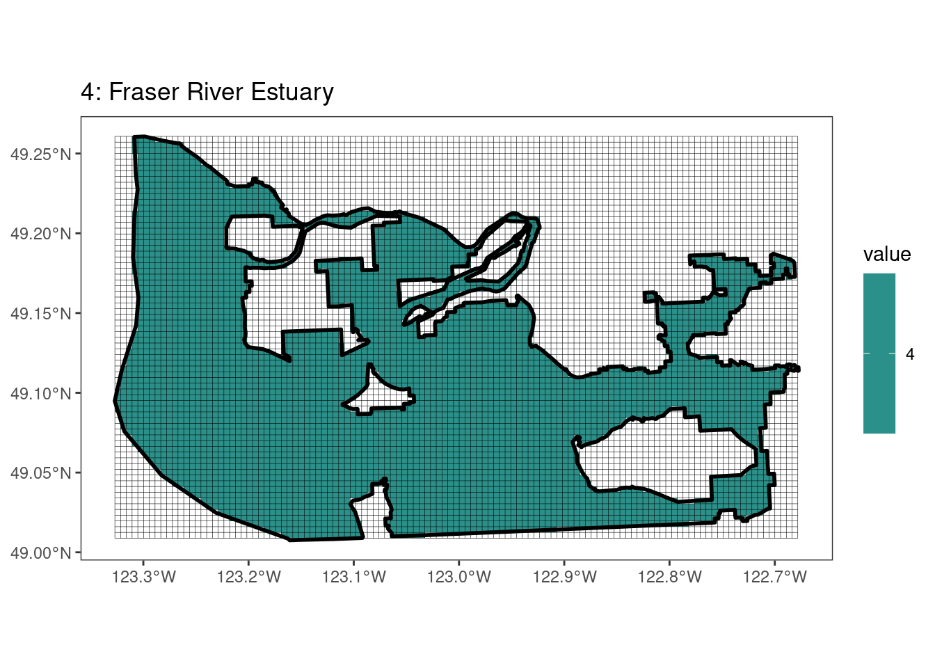
[[2]]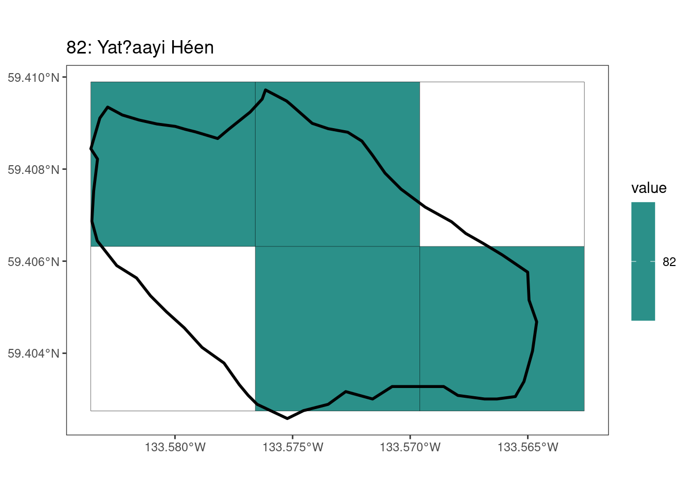
[[3]]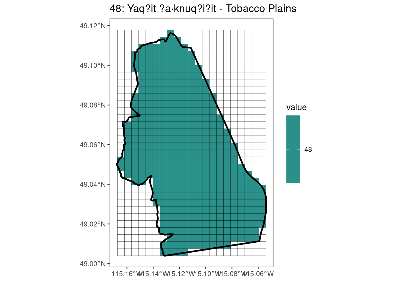
[[4]]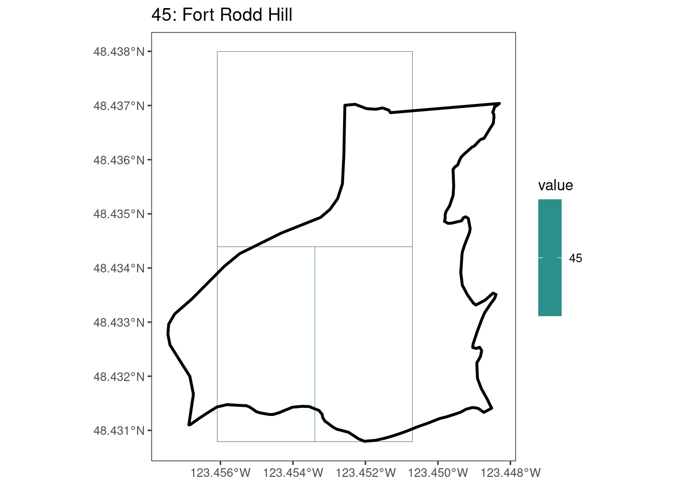
[[5]]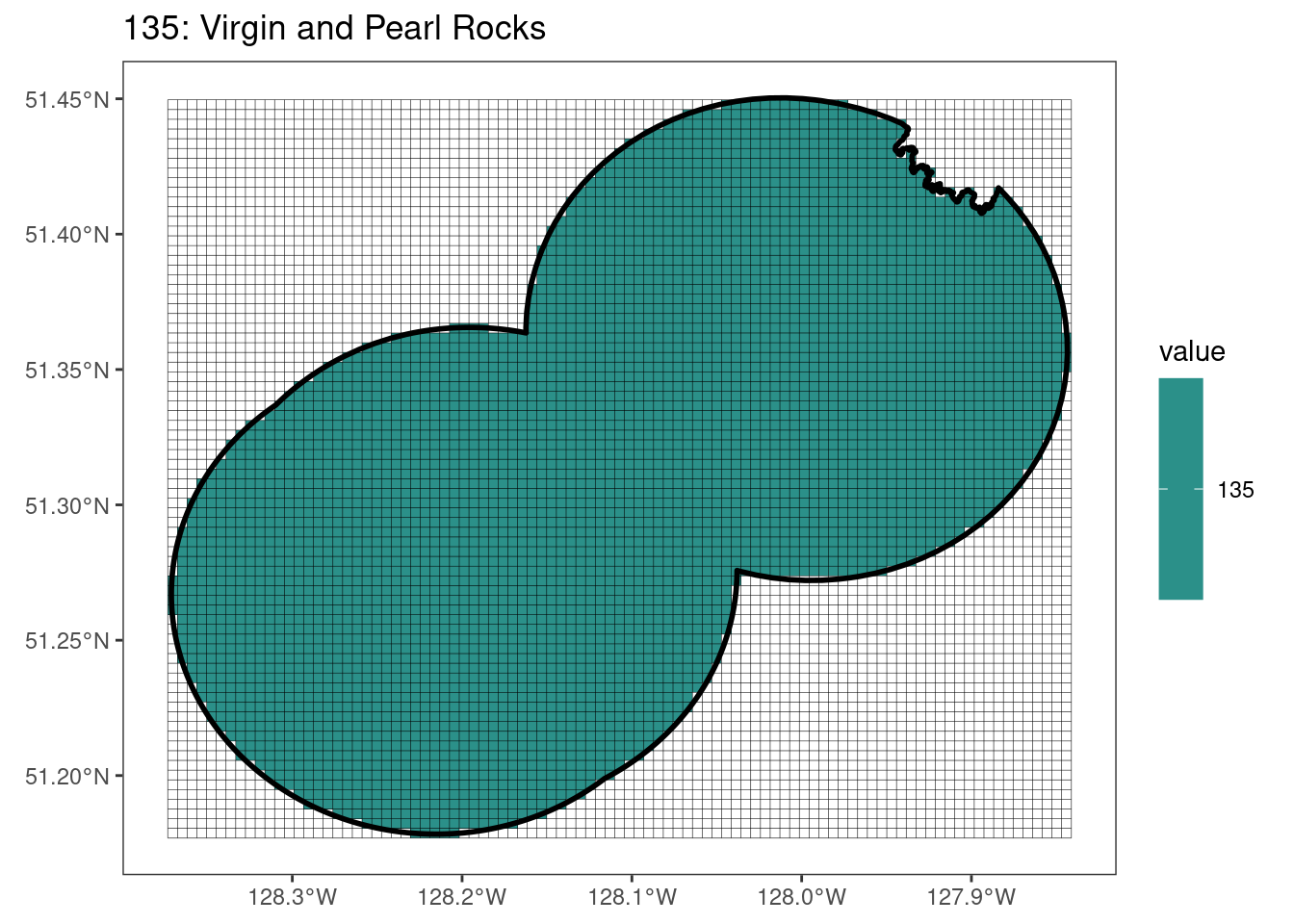
[[6]]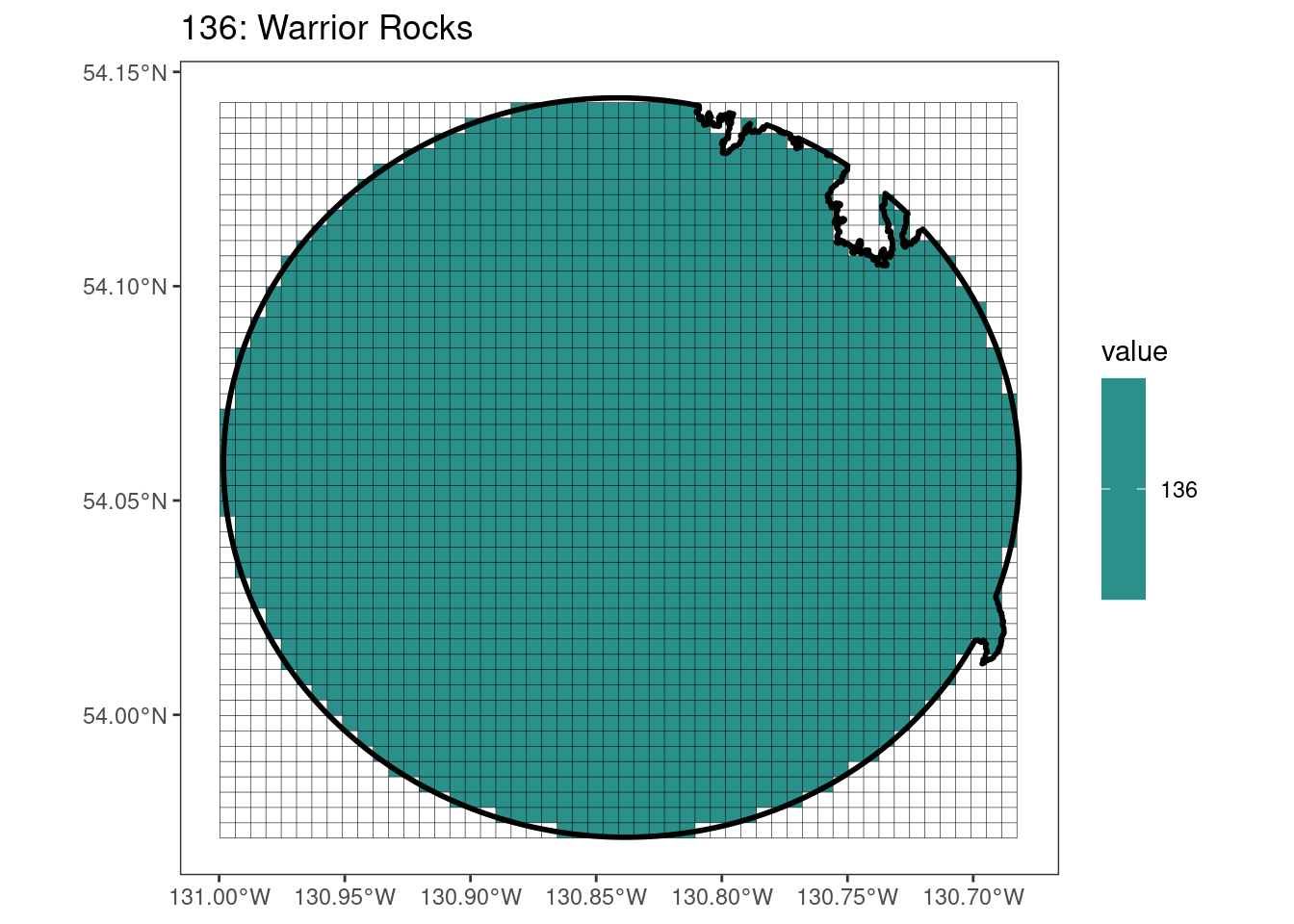
[[7]]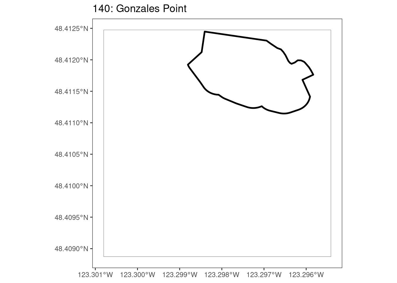
[[8]]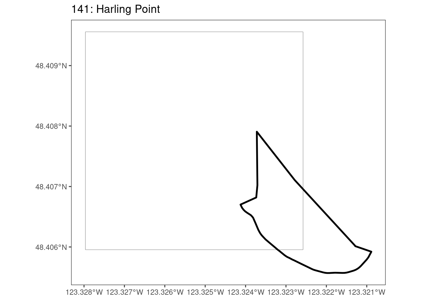
[[9]]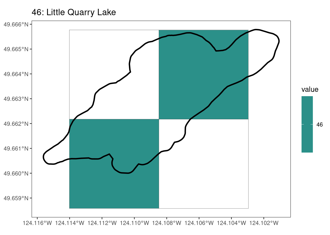
[[10]]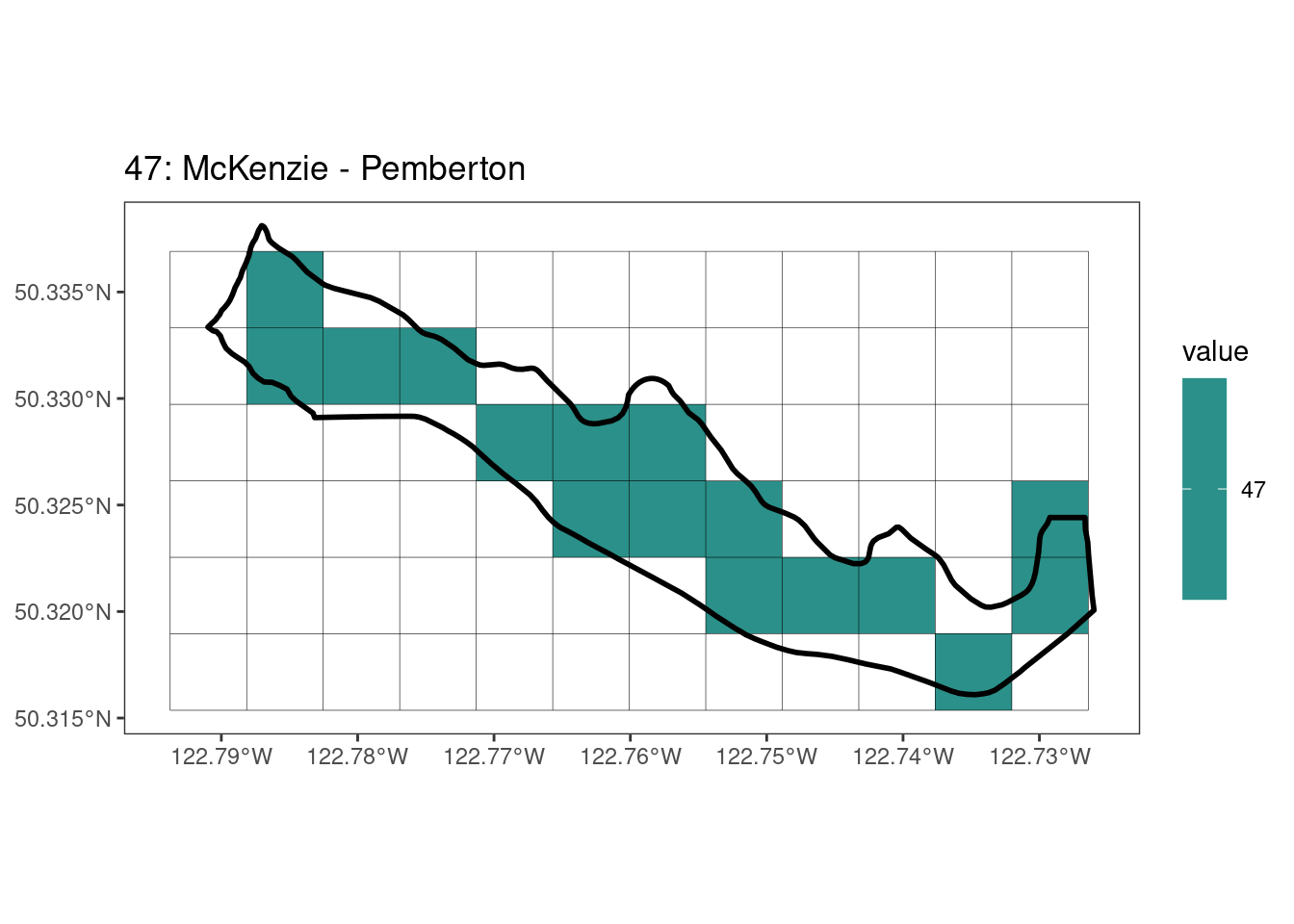
[[11]]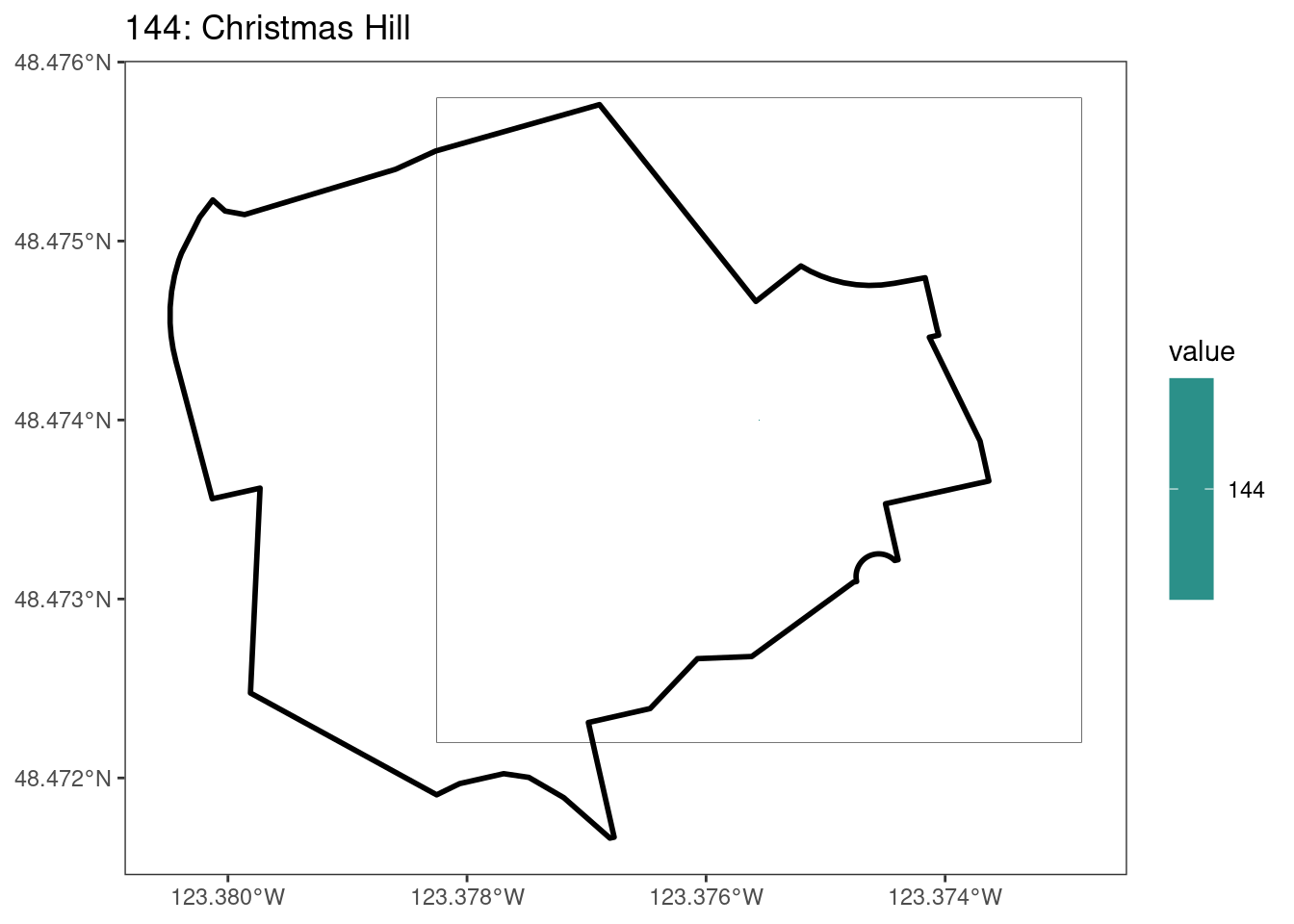
[[12]]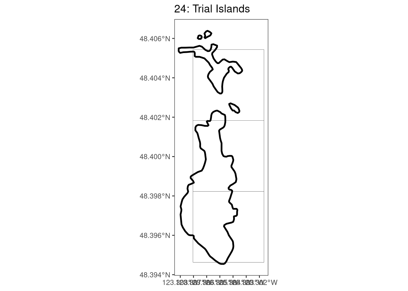
[[13]]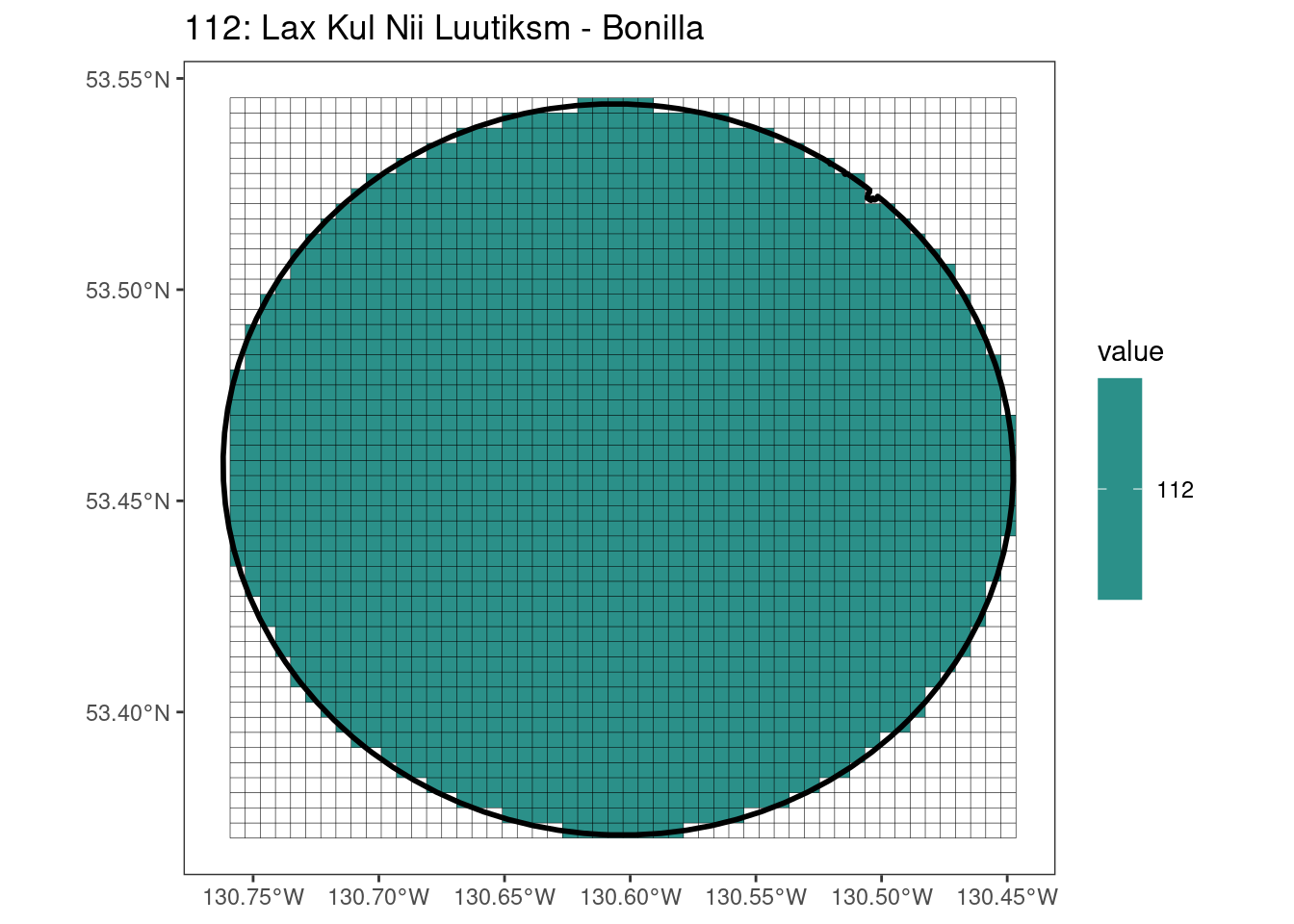
[[14]]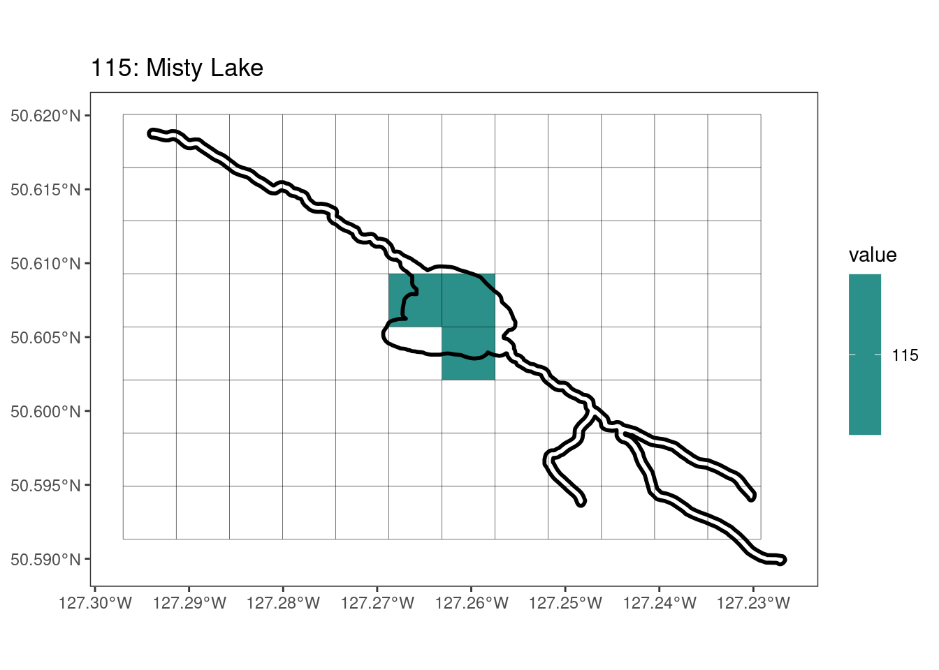
[[15]]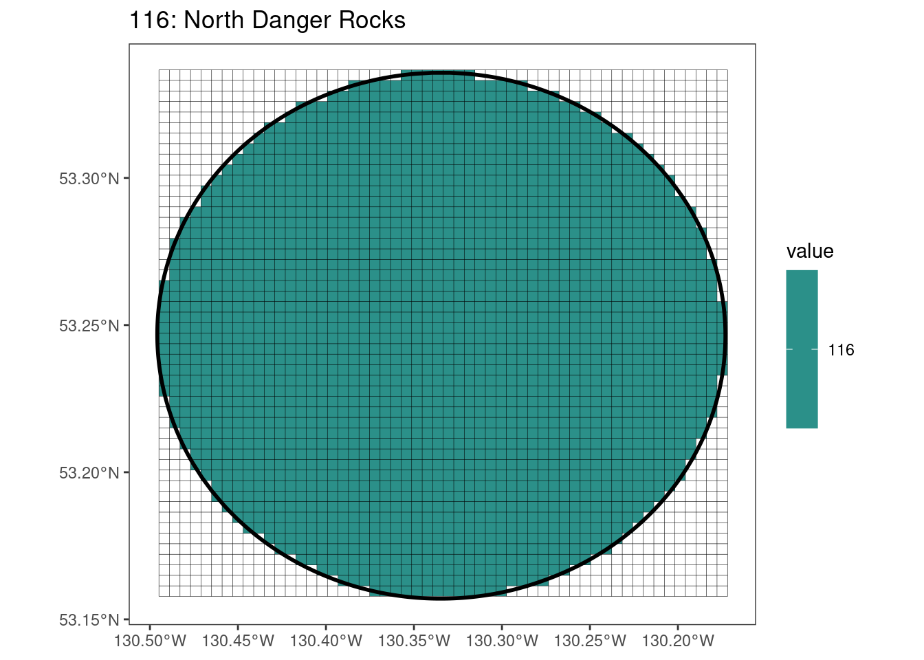
[[16]]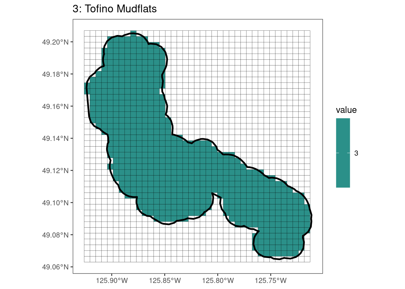
[[17]]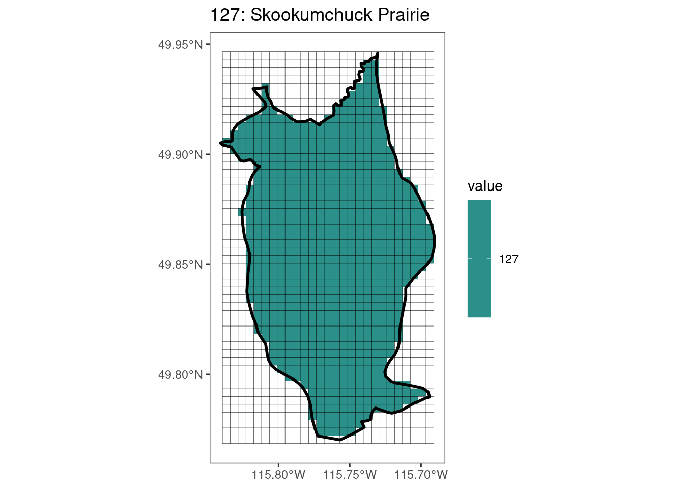
[[18]]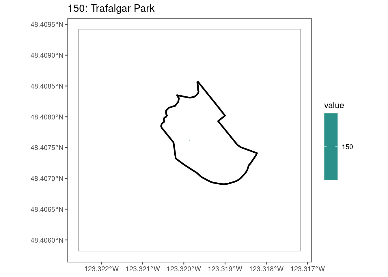
[[19]]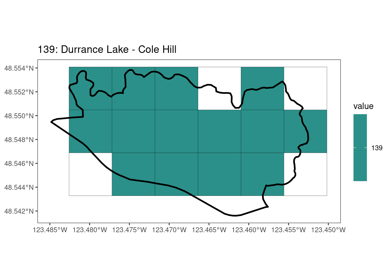
[[20]]
[[21]]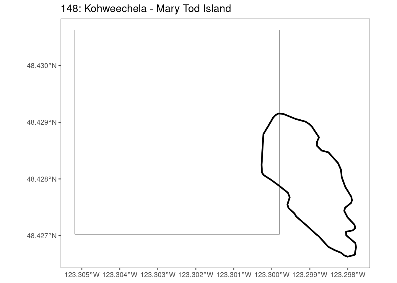
[[22]]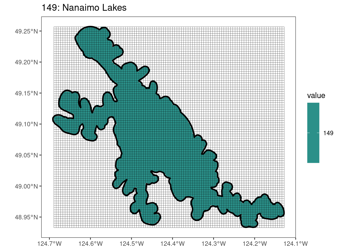
[[23]]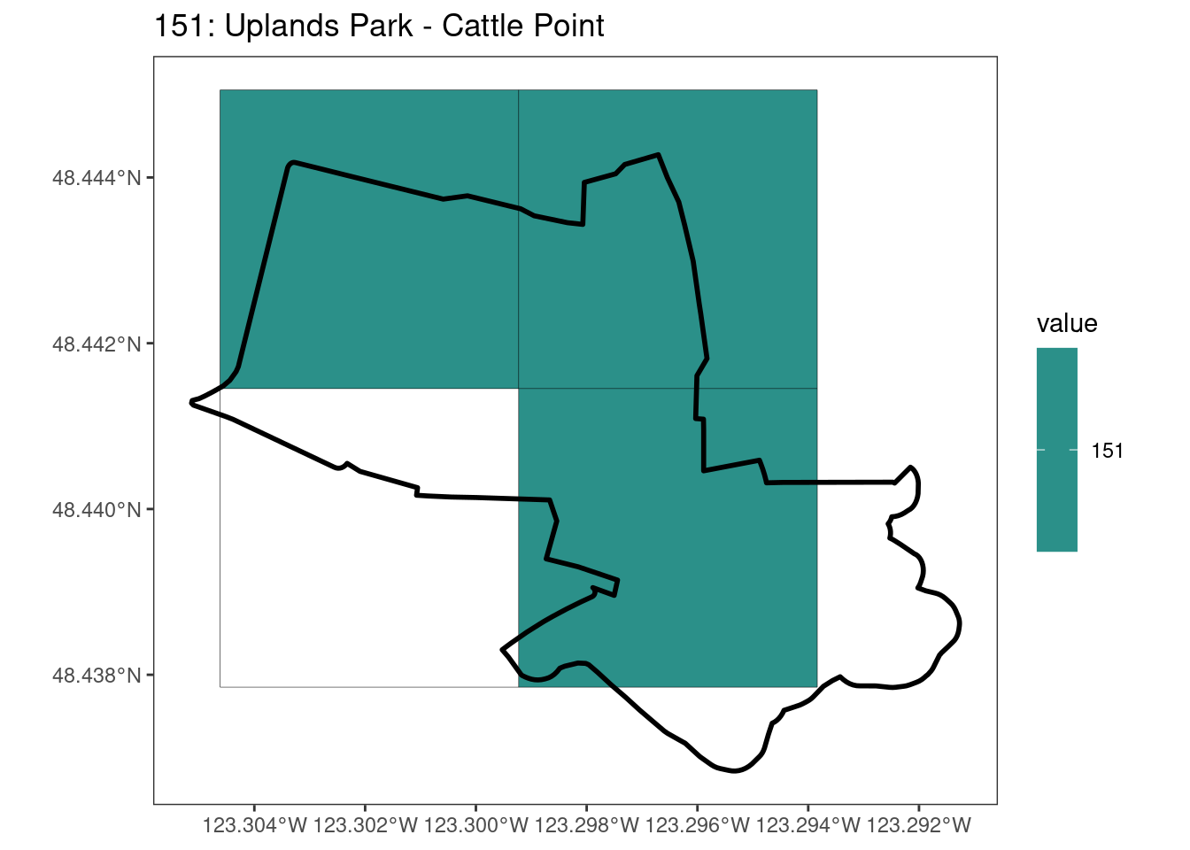
[[24]]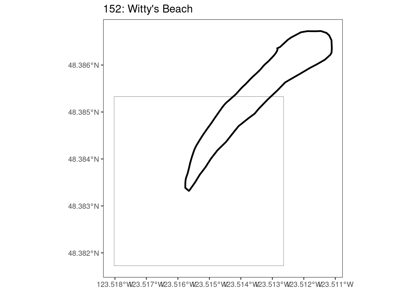
[[25]]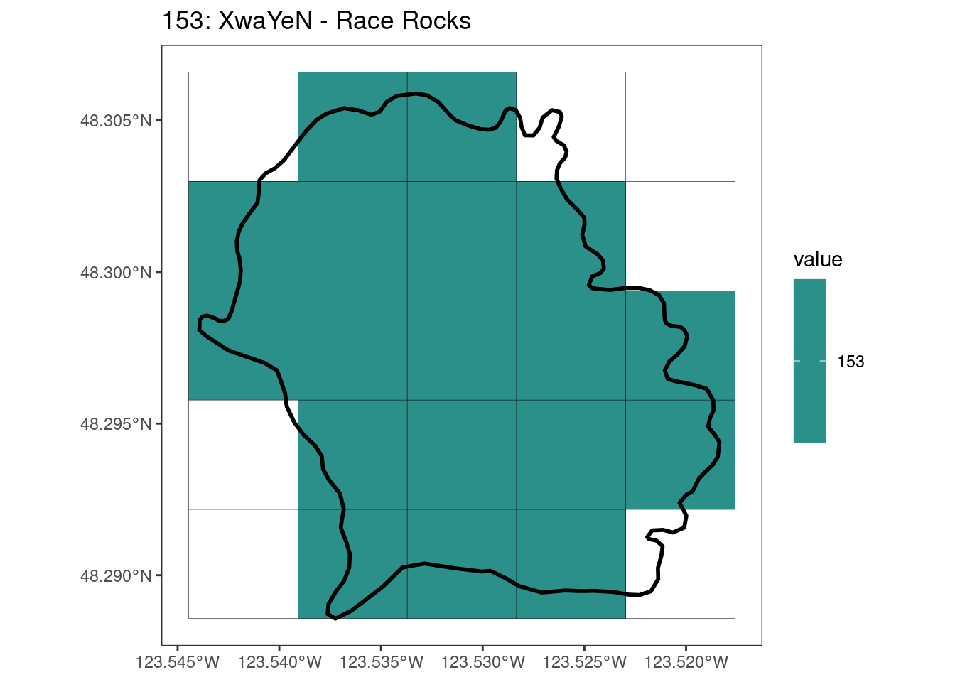
Tip
rasterize all KBAs using touches = T:
# This loop demonstrates some missed rasterized polygons
plots <- foreach(i = 1:length(kba_vect)) %do%
  {
    select_kba <- kba_vect[i, ]

    select_kba_rast <- rasterize(select_kba, ext_rast, "SiteID", touches = T) |>
      crop(select_kba, snap = "out") # good example of crop needing snap = "out"
    select_ext_lines <- as.lines(select_kba_rast)

    ggplot() +
      theme_bw() +
      theme(panel.grid = element_blank()) +
      geom_spatraster(data = select_kba_rast) +
      scale_fill_viridis_c(na.value = NA) +
      geom_spatvector(data = select_ext_lines, linewidth = 0.1) +
      geom_spatvector(
        data = select_kba,
        fill = NA,
        color = "black",
        linewidth = 1
      ) +
      labs(
        title = paste0(
          values(select_kba[, "SiteID"]),
          ": ",
          values(select_kba[, "Name_EN"])
        )
      )
  }
plots
[[1]]
[[2]]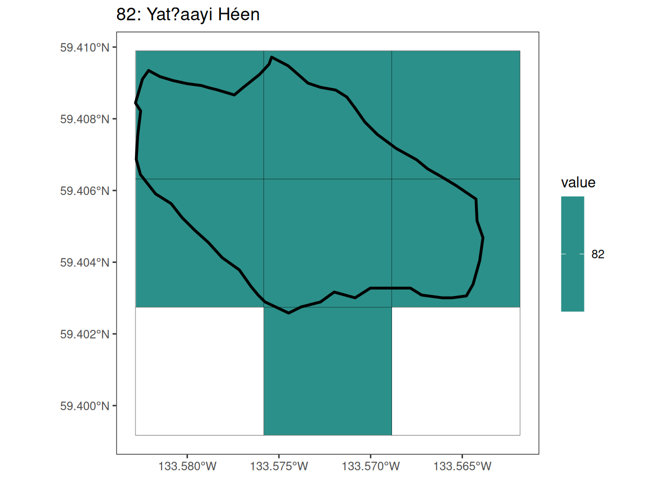
[[3]]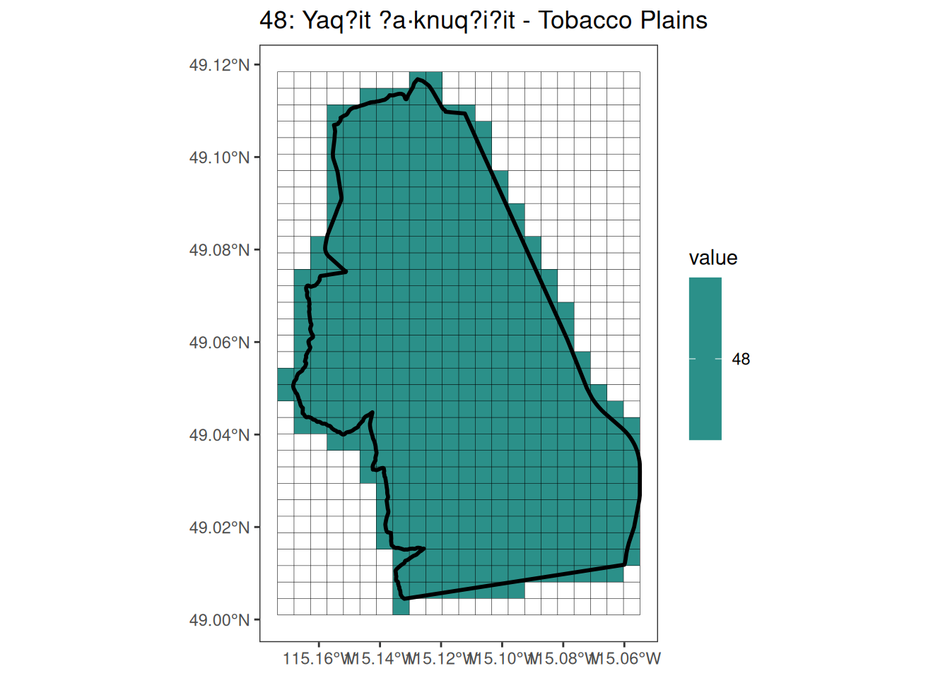
[[4]]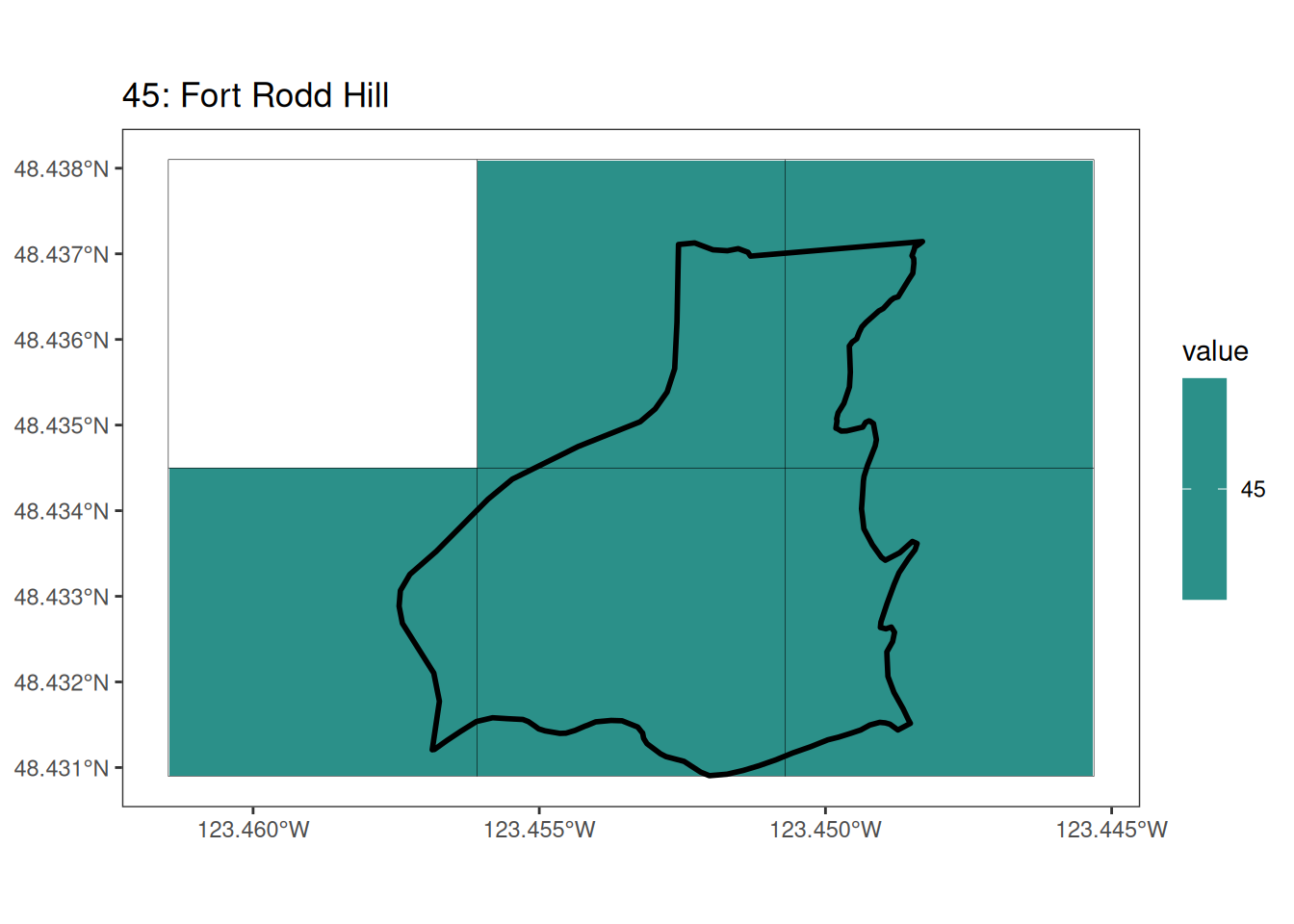
[[5]]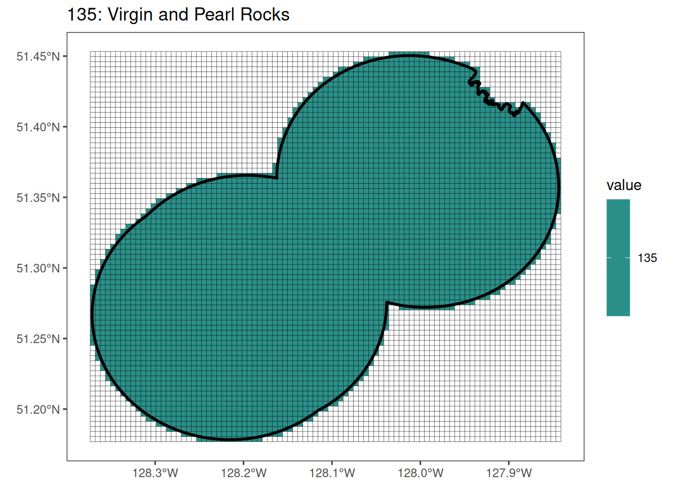
[[6]]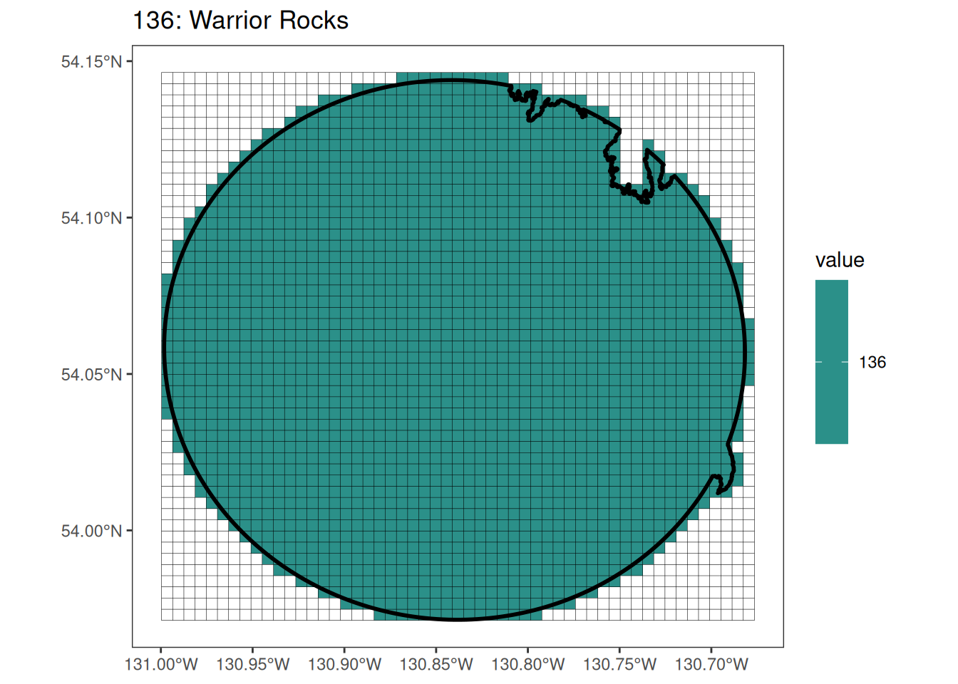
[[7]]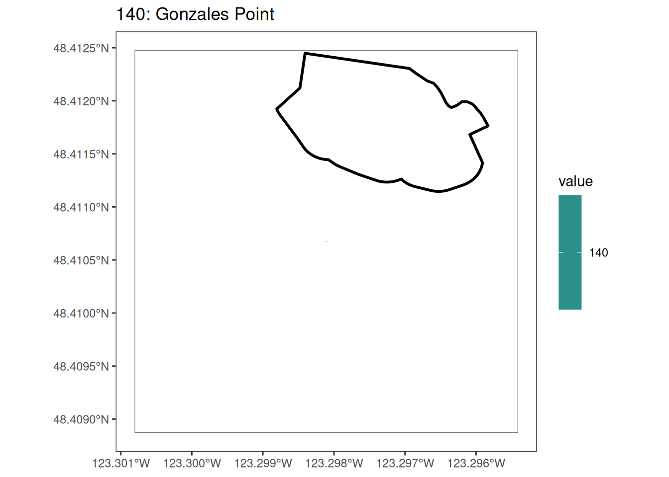
[[8]]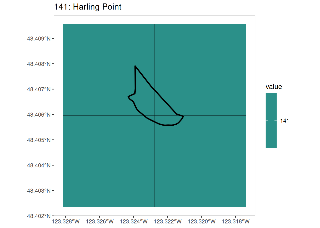
[[9]]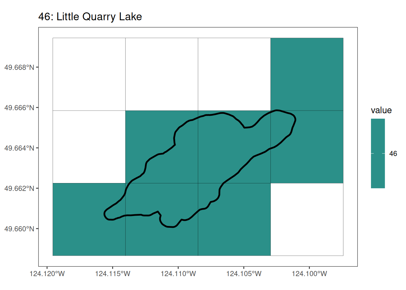
[[10]]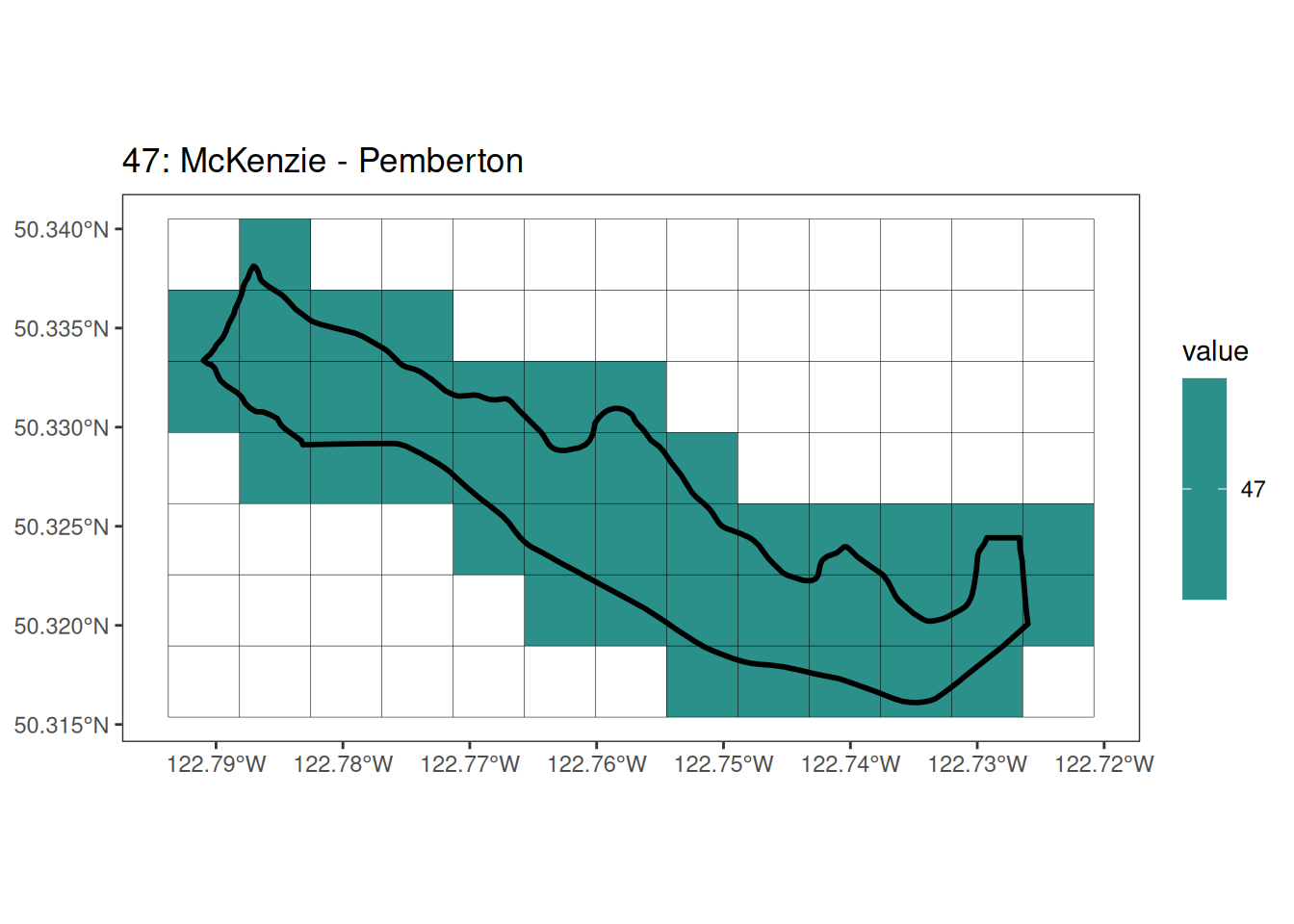
[[11]]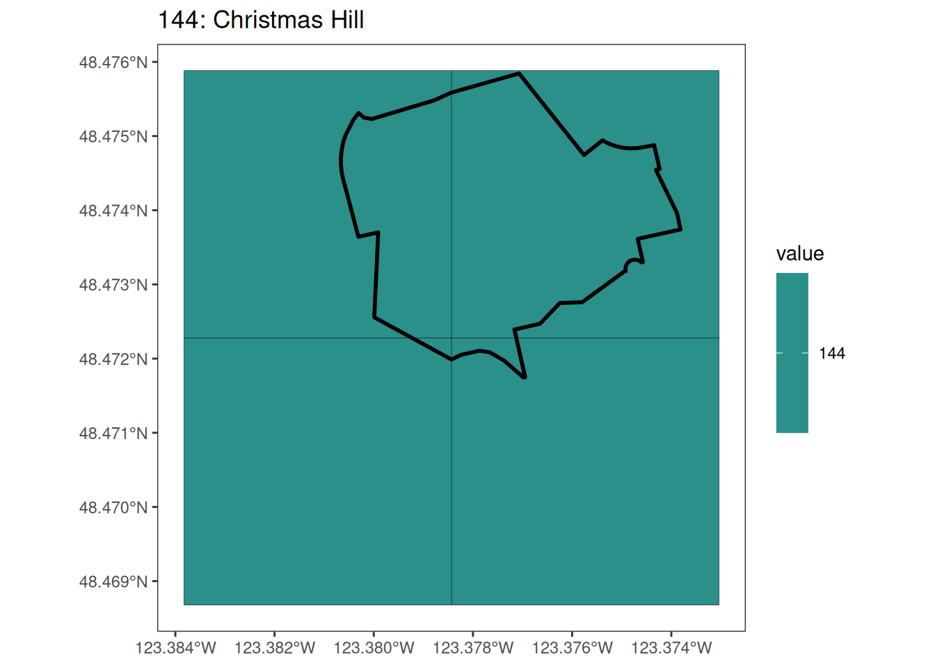
[[12]]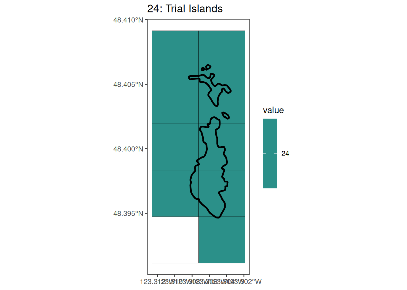
[[13]]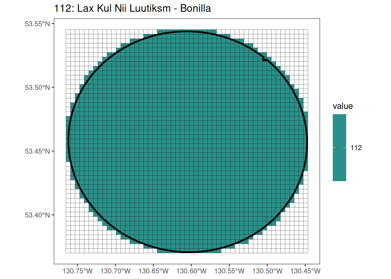
[[14]]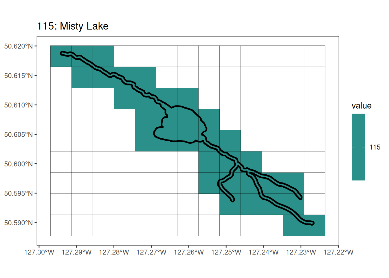
[[15]]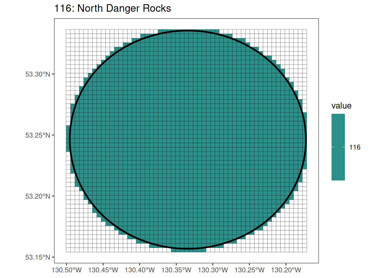
[[16]]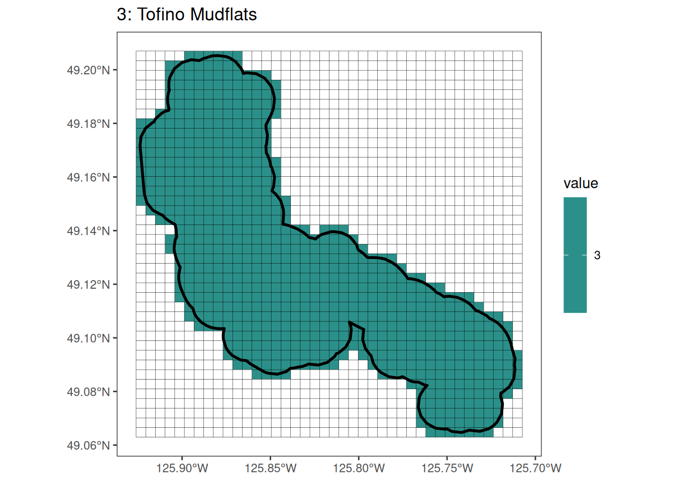
[[17]]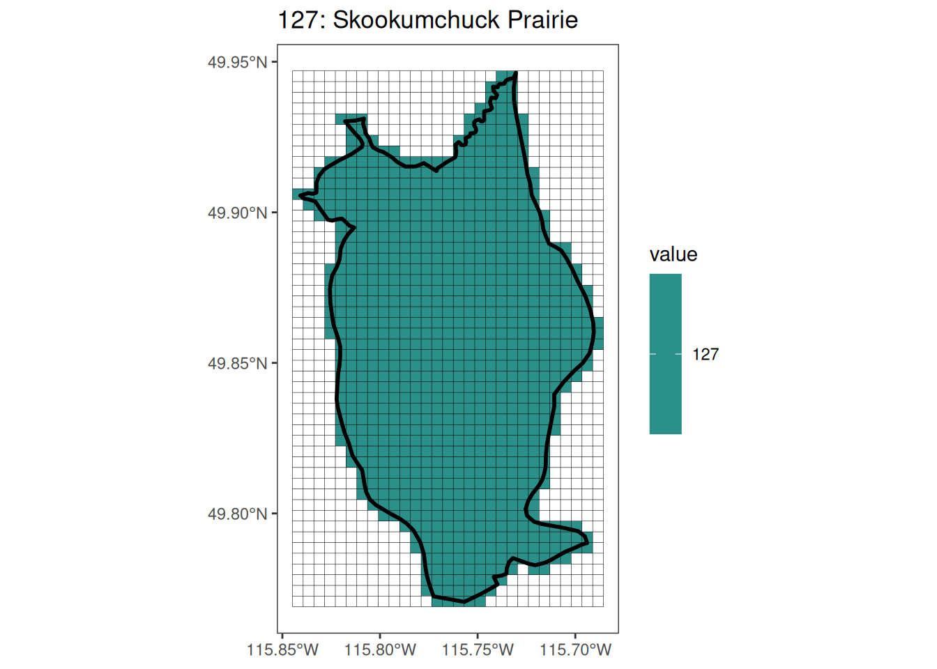
[[18]]
[[19]]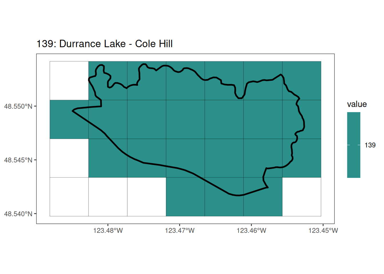
[[20]]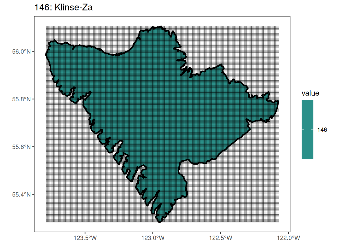
[[21]]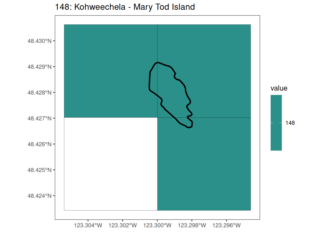
[[22]]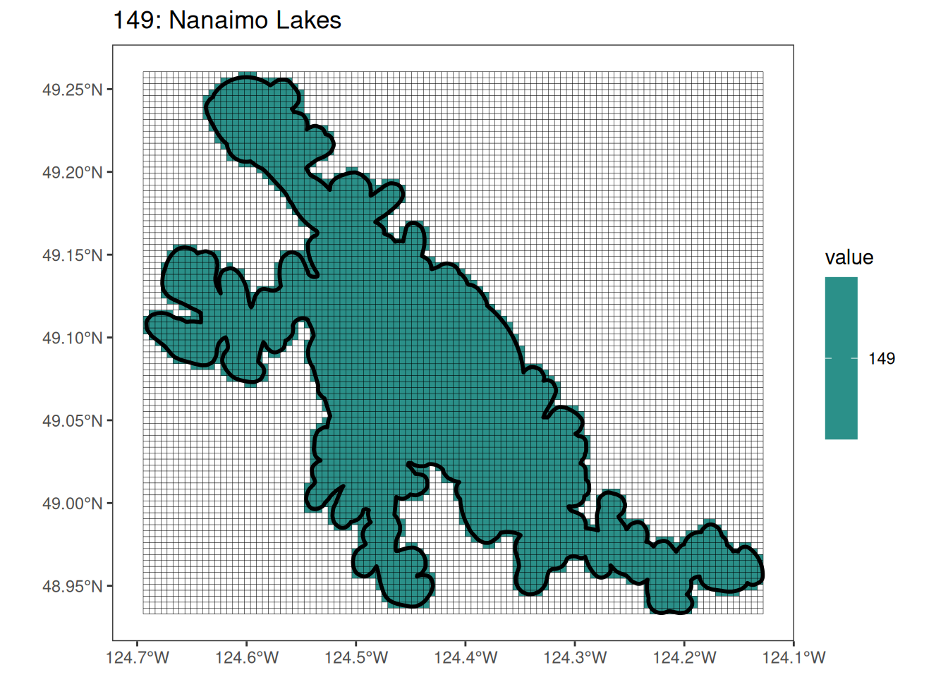
[[23]]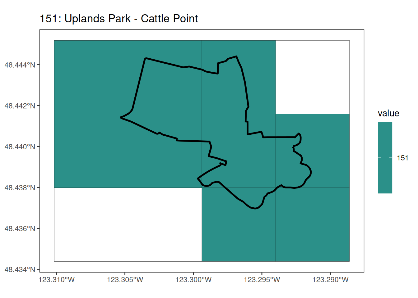
[[24]]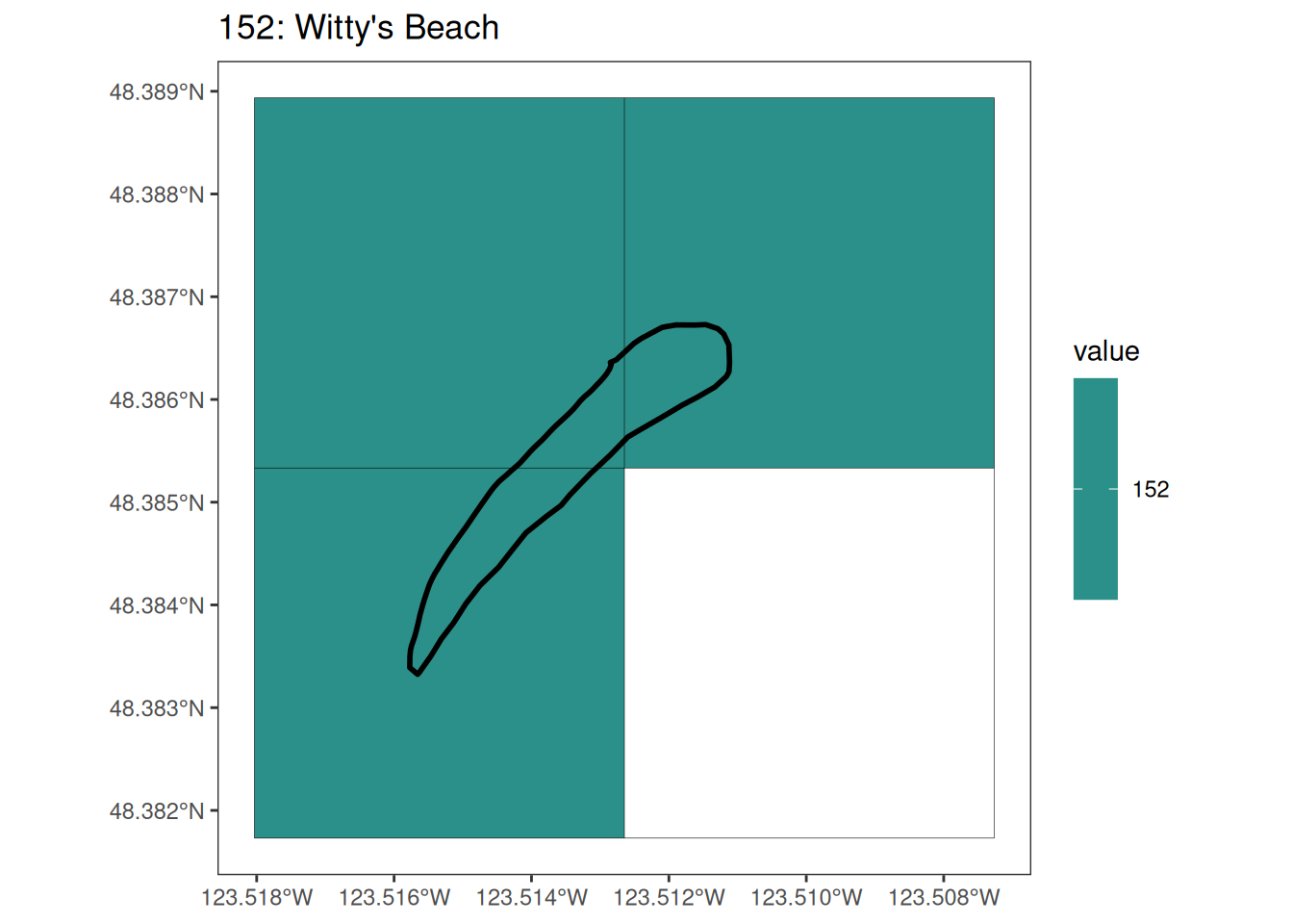
[[25]]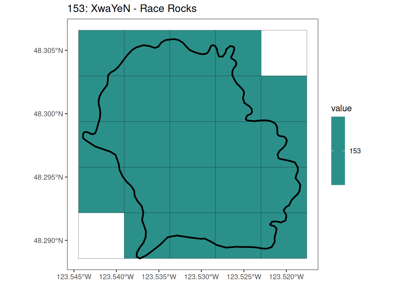
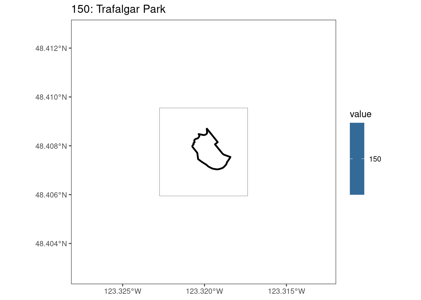
WarningNote: Visualizing single cell raster with tidyterra
After running rasterize on all KBAs, we can find that there are some polygons that become rasterized fully and others than are not.
# loading Key Biodiversity Areas
kba_vect <- vect(here(
  "posts/terra_package_quirks/key_biodiversity_areas/kba.20240514080519.shp"
)) |>
  project("epsg:3005") # reproject to BC Albers

# create empty rast to extent of full KBAs layer
ext_rast <- rast(kba_vect, resolution = c(400))

select_kba <- kba_vect[kba_vect$SiteID == 150, ]

select_kba_rast <- rasterize(select_kba, ext_rast, "SiteID", touches = T) |>
  crop(select_kba)
select_ext_lines <- as.lines(select_kba_rast)

values(select_kba_rast) # has a single value
SiteID
[1,] 150# doesn't visualize the raster cell
ggplot() +
theme_bw() +
theme(panel.grid = element_blank()) +
scale_x_continuous(expand = c(1, 1)) +
scale_y_continuous(expand = c(1, 1)) +
geom_spatraster(data = select_kba_rast) +
# scale_fill_viridis_c(na.value = NA) +
geom_spatvector(data = select_ext_lines, linewidth = 0.1, fill = NA) +
geom_spatvector(
data = select_kba,
fill = NA,
color = "black",
linewidth = 1
) +
labs(
title = paste0(
values(select_kba[, "SiteID"]),
": ",
values(select_kba[, "Name_EN"])
)
)
# does visualize the raster cell
plot(select_kba_rast)
lines(select_ext_lines)
lines(select_kba)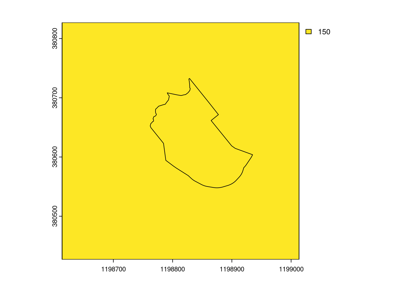
terra::crop unexpectedly misses raster cells
When using terra::crop with SpatRaster and SpatVector inputs, the outputs can be unexpected.
Example
Setup
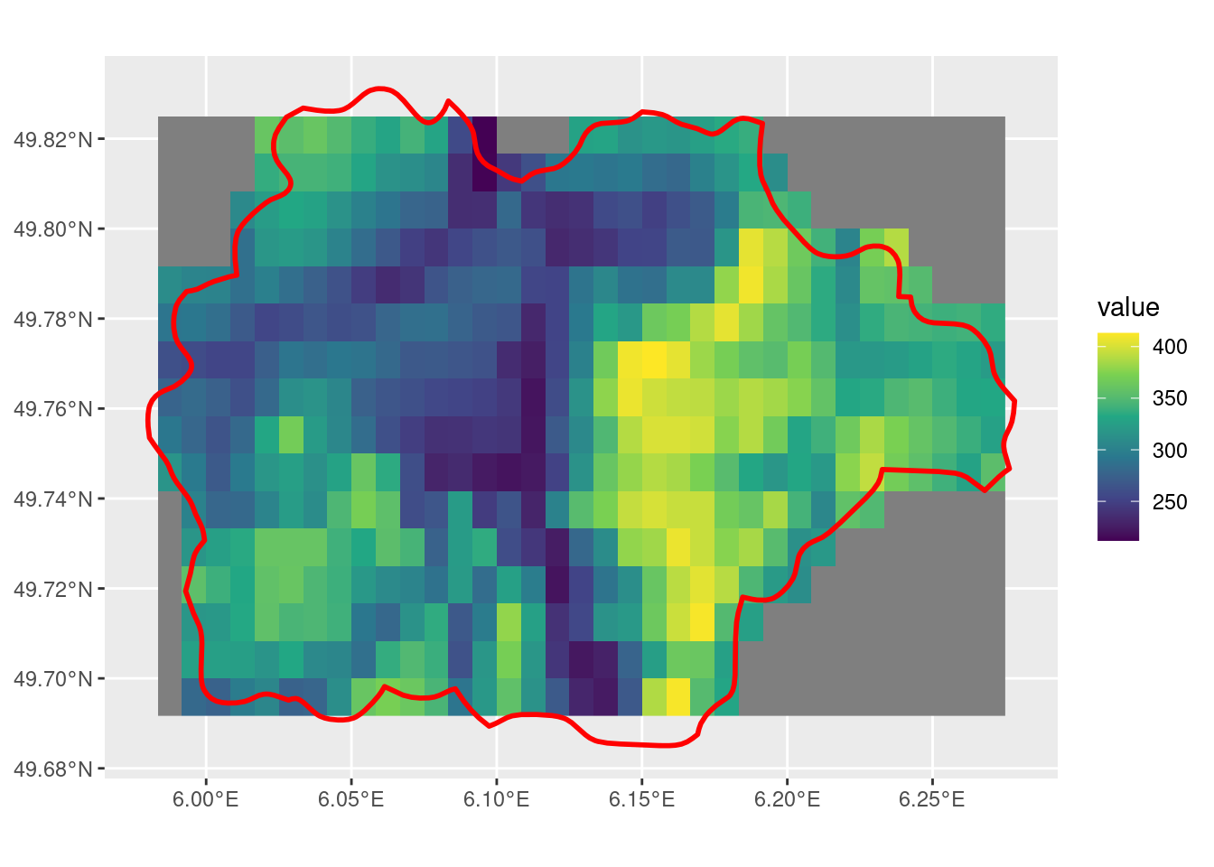
Setting up the example scenario, where we crop the larger raster by a vector polygon.
# sample raster
r <- rast(system.file("ex/elev.tif", package = "terra"))
# sample vector
p <- vect(system.file("ex/lux.shp", package = "terra"))
sel_p <- p[p$NAME_2 == "Mersch"]

ggplot() +
  geom_spatraster(data = r) +
  scale_fill_viridis_c() +
  geom_spatvector(data = sel_p, linewidth = 1, fill = NA, color = "red")
default crop
Note that the default settings for crop with x as SpatRaster and y as SpatVector outputs a SpatRaster that is the size of the extent of the input SpatVector. Also note that there are some cells that the SpatVector touches but is not included in the output, which is related to the first issue outlined in this post.
default_r <- crop(r, sel_p)

ggplot() +
  geom_spatraster(data = default_r) +
  scale_fill_viridis_c() +
  geom_spatvector(data = sel_p, linewidth = 1, fill = NA, color = "red")
crop with touches = F
Note that touches = F doesn’t change the output in this case, still with some cells that do have the SpatVector overlapping that do not get included.
t_r <- crop(r, sel_p, touches = F)

ggplot() +
  geom_spatraster(data = t_r) +
  scale_fill_viridis_c() +
  geom_spatvector(data = sel_p, linewidth = 1, fill = NA, color = "red")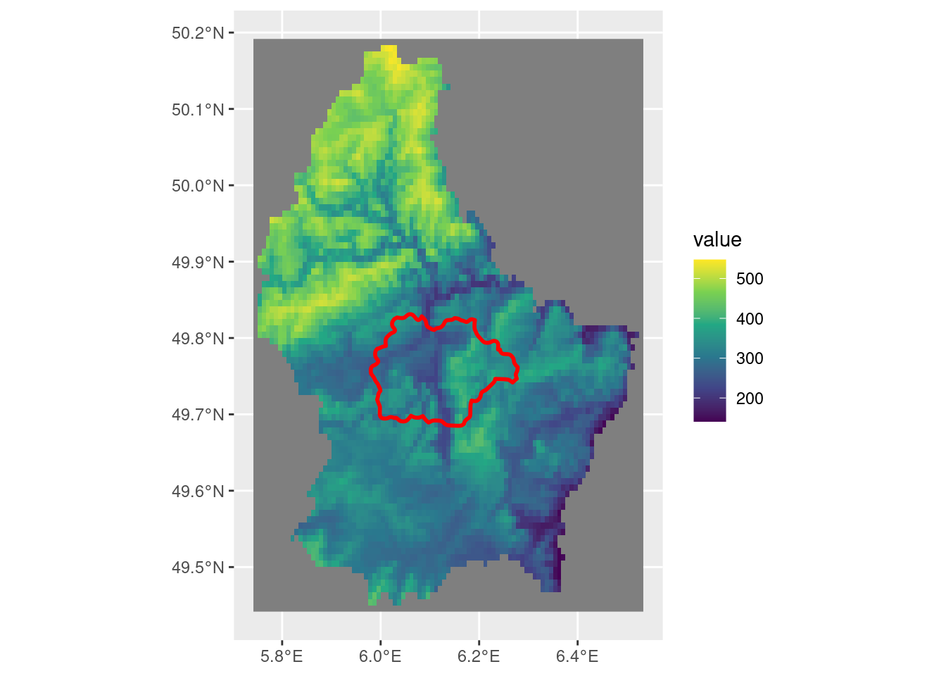
crop with mask = T
With mask = T, the cells that intersect with the SpatVector are given a value, while those that do not have a NA value. However, this doesn’t fix the few cells that do have the SpatVector overlapping that do not get included.
m_r <- crop(r, sel_p, mask = T)

ggplot() +
  geom_spatraster(data = m_r) +
  scale_fill_viridis_c() +
  geom_spatvector(data = sel_p, linewidth = 1, fill = NA, color = "red")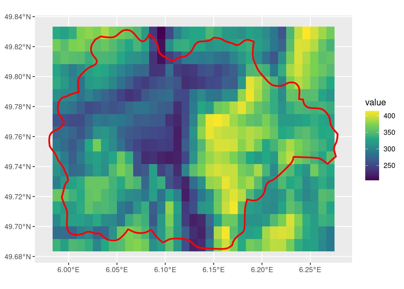
crop with mask = T and touches = F
Having both mask = T and touches = T leads to fewer cells being selected. However, the cells along the edge of the SpatVector may or may not be selected, not a consistent behaviour that I would expect.
tm_r <- crop(r, sel_p, mask = T, touches = F)

ggplot() +
  geom_spatraster(data = tm_r) +
  scale_fill_viridis_c() +
  geom_spatvector(data = sel_p, linewidth = 1, fill = NA, color = "red")
crop with snap = "in"
The default value is snap = "near". This is the parameter that is responsible for controlling this behaviour around the raster cells that overlap with the SpatVector but are not included in the crop. Depending on the geometry of the raster and the vector, this default can lead to some unexpected results.
in_r <- crop(r, sel_p, snap = "in")

ggplot() +
  geom_spatraster(data = in_r) +
  scale_fill_viridis_c() +
  geom_spatvector(data = sel_p, linewidth = 1, fill = NA, color = "red")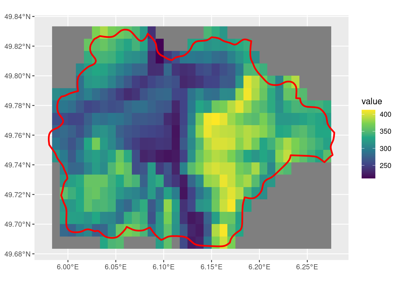
crop with snap = "out"
This finally fixes the issue with the full SpatVector extent being covered by the output SpatRaster.
out_r <- crop(r, sel_p, snap = "out")

ggplot() +
  geom_spatraster(data = out_r) +
  scale_fill_viridis_c() +
  geom_spatvector(data = sel_p, linewidth = 1, fill = NA, color = "red")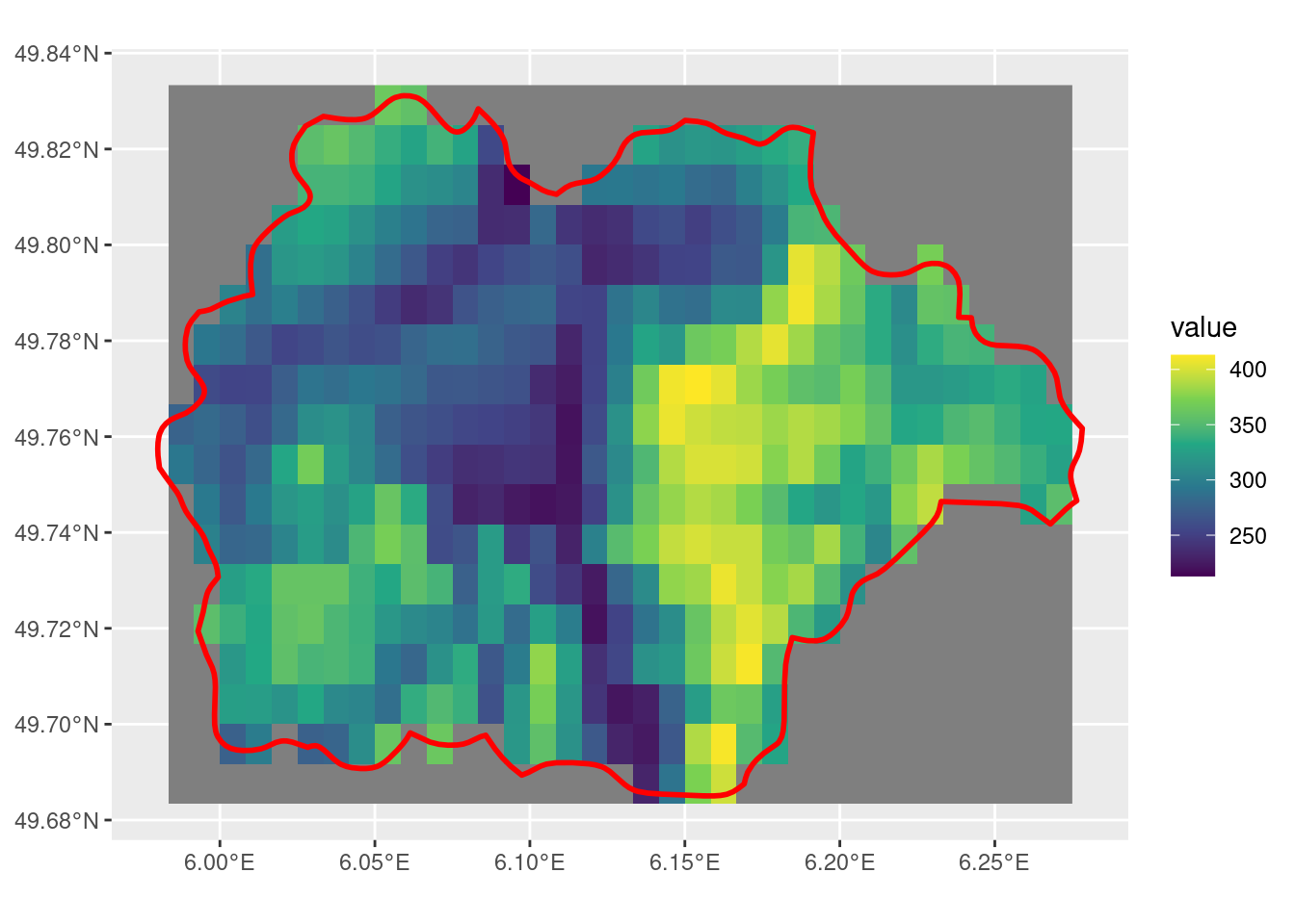
crop with snap = "in" and mask = T
The snap = "in"parameter by itself doesn’t seem to do what I would expect. While it does select fewer cells compared to snap = "out", there are still many that are along the edge of the SpatVector that I would have expected to be removed, with this parameter.
min_r <- crop(r, sel_p, snap = "in", mask = T)

ggplot() +
  geom_spatraster(data = min_r) +
  scale_fill_viridis_c() +
  geom_spatvector(data = sel_p, linewidth = 1, fill = NA, color = "red")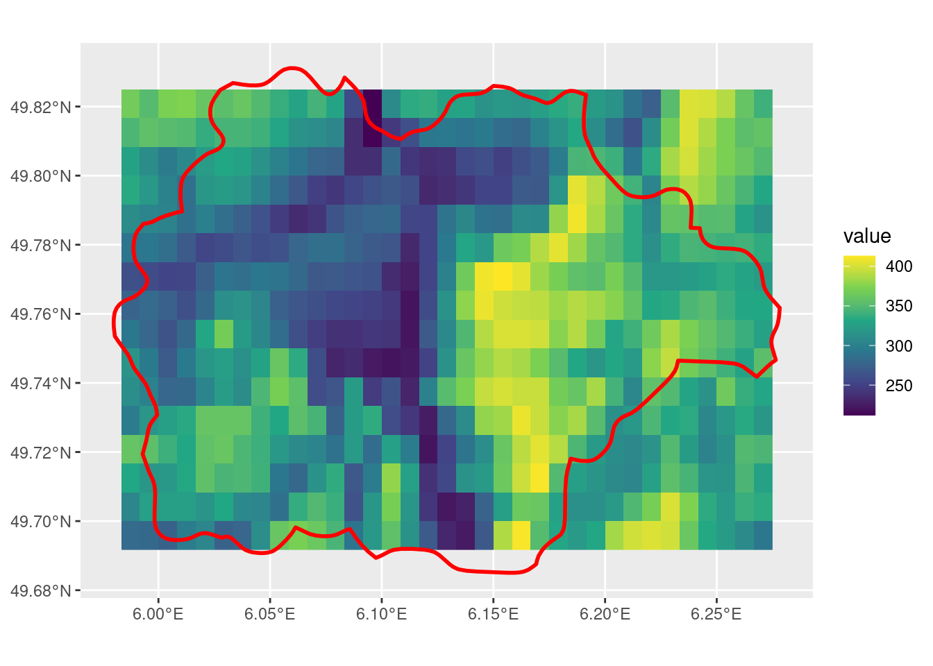
crop with snap = "in", mask = T and touches = F
With touches = F, the crop output is fewer than with the same parameters. The behaviour of the cells along the edge of the SpatVector is still inconsistent to what I would find intuitive.
tmin_r <- crop(r, sel_p, mask = T, snap = "in", touches = F)

ggplot() +
  geom_spatraster(data = tmin_r) +
  scale_fill_viridis_c() +
  geom_spatvector(data = sel_p, linewidth = 1, fill = NA, color = "red")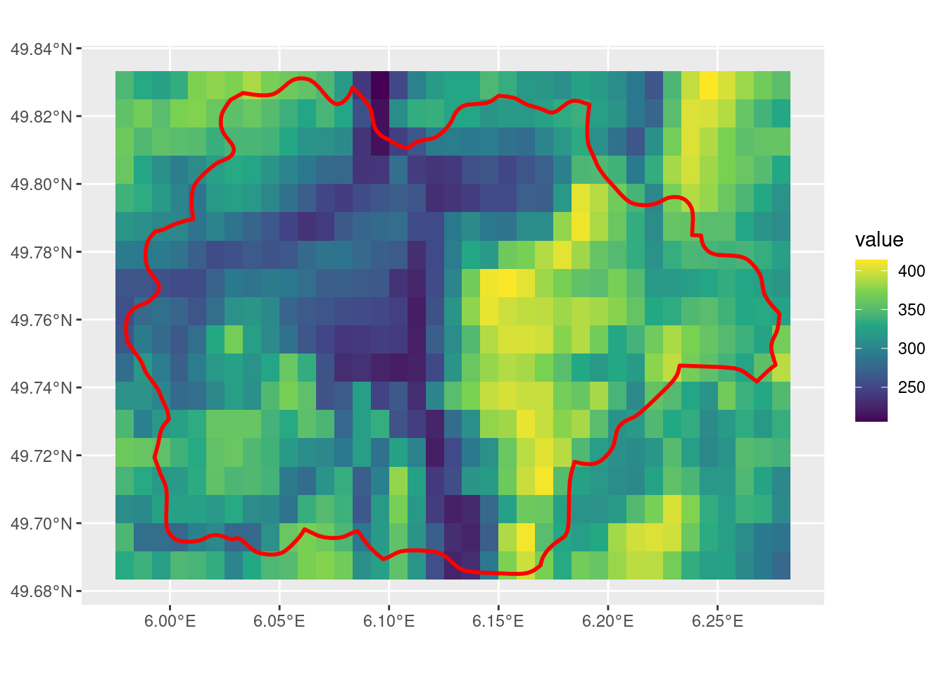
crop with snap = "out" and mask = T
Finally, using crop with these parameters delivers the most intuitive result from using the function. This outputs a SpatRaster that has cells with values for all that overlap with the SpatVector.
mout_r <- crop(r, sel_p, snap = "out", mask = T)

ggplot() +
  geom_spatraster(data = mout_r) +
  scale_fill_viridis_c() +
  geom_spatvector(data = sel_p, linewidth = 1, fill = NA, color = "red")