sharkabc3d: 3D Marine Spatial Analysis for Sharks and Rays

Spatial

Tech

Data Visualization

An open-source R package for analysing shark, ray, and chimaera habitat in three dimensions — keeping depth in the picture so species ranges, environmental conditions, and fishing pressure can be compared by volume rather than area alone.

Author

Jay Matsushiba

Published

June 18, 2026

Modified

June 18, 2026

At a glance

An open-source R package for analysing shark, ray, and chimaera habitat in three dimensions. Most marine GIS flattens the ocean into a 2D plane. sharkabc3d keeps depth in the picture, so that species ranges, environmental conditions, and fishing pressure can be compared by volume rather than by area alone.

My role: Lead developer and first author. I led the spatial analysis and R development on several lab projects, working as the scientific software developer on each, then brought that work together into one documented, tested package. I designed the architecture, wrote the documentation and tests, trained collaborators to use it, and presented the work at Sharks International 2026.
What it is: An R package built on terra and sf. It rasterizes species ranges and fishery footprints onto a shared, bathymetry-aware grid, then computes their 3D volume overlap through raster algebra.
Why it matters: Fisheries operate at specific depths depending on gear type. A species and a fishery can overlap completely on a 2D map yet barely meet in 3D, because the species holds a depth refuge below the gear. Quantifying that gap requires working in volume, not area.
Demonstrated at scale: At Sharks International 2026 I showed the same small set of functions carrying three very different analyses. It scaled from select species and fisheries on the Bangladesh shelf (Haque et al.), to temperature and dissolved oxygen profiles for 1,213 chondrichthyan species pulled from IUCN Red List ranges and World Ocean Atlas 2023 climatologies (Aitchison et al., VanderWright et al.), to depth-stratified fishing effort across the entire Japan EEZ from Global Fishing Watch (Matsushiba et al.). One species or the full global list, the workflow does not change.
Data sources: IUCN Red List, GEBCO bathymetry, World Ocean Atlas 2023, Global Fishing Watch, and custom spatial layers such as marine protected areas.
Status: In active development. The core volume, extraction, World Ocean Atlas, and plotting functions are implemented and tested. Presented at Sharks International 2026 in Sri Lanka.

sharkabc3d on GitHub

Context

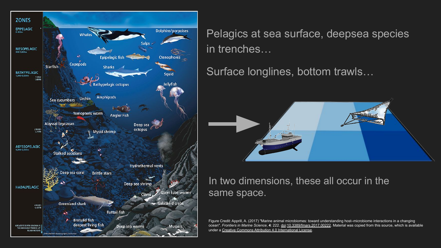Ocean depth zones collapsed into a single 2D plane From the talk: the ocean spans depth zones from the epipelagic surface to the hadal trenches, but a 2D map collapses surface longlines, bottom trawls, and the species between them into the same space. (Depth-zone figure: Apprill 2017, CC BY 4.0.)

Sharks, rays, and chimaeras live in three dimensions, but most conventional GIS workflows represent space as a flat plane. In that representation, pelagic species near the surface, deep sea species in trenches, and everything in between are flattened into the same space. The same goes for fishing: surface longlines and bottom trawls are treated as if they work the same part of the ocean.

These conventional GIS approaches that simplify space into the 2D plane cannot capture the range of depths of marine habitat and anthropogenic activity, and therefore cannot represent the depth-specific patterns of threat exposure to a given species. I have worked on this issue on a number of past projects with the Dulvy Lab: 3D fisheries overlap in Bangladesh, environmental data extraction at depth from oceanographic datasets, and analyzing depth refuge for deep sea chondrichthyans. As I worked, I found myself reusing chunks of code and copy-pasting across projects. But scattered code is hard to reuse and hard to verify, so I could never be sure it would behave the same way from one project to the next.

I decided to create sharkabc3d to bring these methods together into a single, documented, tested R package, so that the analyses can be reproduced and rerun as new data, species, or parameters come along.

My Role

I am the lead developer and first author of sharkabc3d, working in the Marine Biodiversity and Conservation Lab (Dulvy Lab) at Simon Fraser University. On several lab projects I was the scientific software developer, leading the spatial analysis in R: Rachel Aitchison’s environmental extraction work, Wade VanderWright’s analyses, and Dr. Alifa Haque’s Bangladesh fisheries study. Each analysis worked, but lived as its own set of scripts tied to a single paper. sharkabc3d brings that work together into one reproducible toolkit, so the methods can be rerun on new data, species, or regions instead of rebuilt each time.

My job was to take the analytical ideas proven across those projects and turn them into software: a coherent set of functions with a consistent data model, documentation, test coverage, and worked examples. I designed the stacked-raster approach that underpins the volume calculations, wrote the World Ocean Atlas and Global Fishing Watch utilities, built the plotting functions, and prepared the package and presentation for Sharks International 2026. I also run the project as a shared resource rather than a personal one. I train collaborators to use the package and coordinate their work on the codebase, so these methods are something a team can pick up and depend on, not just something I can run myself. The point of all this is leverage: I solve the software problems once so that everyone using these methods benefits at the same time, and my collaborators get to spend their time on the science instead of the tooling.

Approach

My core idea takes three ingredients: an outline of where a feature occurs (for example a species range from the IUCN Red List, or a fishing ground mapped from fisher interviews), a depth minimum and maximum, and bathymetry to say how deep the seafloor actually is.

A shared, bathymetry-aware stacked grid spatial model. I built every analysis on a stacked-raster approach. I rasterize polygons onto a common grid where each cell stores presence plus the shallowest and deepest depths the feature occupies, clamped to the seafloor. In previous approaches, I used intermediate hex or vector grids to summarise across spatial layers, like environmental layers or species range polygons. In this package, I avoid use of the intermediate hex or vector grids and lean on terra’s optimised raster operations, which delivered a significant decrease in compute time. I first developed this approach for the Bangladesh fisheries analysis and generalised it here with this package.

Volume overlap through raster algebra. Once two features sit on the same grid, I compute the 3D volume of each, and the volume where they intersect, per cell. Volume is cell area multiplied by the depth interval occupied, summed across the grid. This is what reveals a depth refuge: where a species sits below the depth a gear can reach, the horizontal overlap counts for nothing in 3D.

Depth-stratified environmental data. Multi-depth oceanographic rasters, such as World Ocean Atlas temperature at its standard depth levels, follow a {variable}_depth={value} layer-naming convention. My downstream functions parse those names to select the correct layers for a given depth window, so I can summarise environmental conditions across exactly the depths a species actually uses, not just at the surface.

Depth-aware fishing pressure. I turn apparent fishing effort from Global Fishing Watch into a multi-layer raster, one layer per gear type, then assign it to depth bands (pelagic, benthic, midwater) using bathymetry and a gear-to-depth lookup. This places fishing pressure in the same 3D frame as the species. I kept the gear-to-depth lookup as user-provided, since the characteristics of fisheries differ greatly regionally.

What the package does

flowchart TD
    %% External data sources
    iucn[IUCN Red List<br/>API + shapefile]:::src
    gebco[GEBCO bathymetry]:::src
    woa[WOA NetCDFs]:::src
    gfw[GFW API]:::src
    custom[Custom shapefiles<br/>MPAs, fisheries,<br/>other workflows]:::src

    %% Blackbox: package functions and workflow
    pkg[["sharkabc3d"]]:::fn

    iucn --> pkg
    gebco --> pkg
    woa --> pkg
    gfw --> pkg
    custom --> pkg

    %% Outputs
    pkg --> masked[(Environmental<br/>raster stack for species)]:::out
    pkg --> summary[(Environmental<br/>variable<br/>summary table)]:::out
    pkg --> overlap_rast[(Overlap volume between<br/>species and fisheries)]:::out

    classDef src  fill:#5a3e1f,stroke:#d4a373,color:#fce5cd,stroke-width:1px
    classDef fn   fill:#2a2a2a,stroke:#888888,color:#e8e8e8,stroke-width:1px
    classDef data fill:#0f2942,stroke:#7eb6e6,color:#cfe2f3,stroke-width:1px
    classDef out  fill:#3d3618,stroke:#d4c25e,color:#fff2cc,stroke-width:1px

I organised the package around a small number of reusable functions. The main groups:

Loading and preparing inputs: load_bathymetry() for GEBCO bathymetry, fetch_species_assessments() to query the IUCN Red List API for taxonomy, Red List category, and depth limits, and fill_missing_depths() to repair and infer missing depth values from genus-level means.
Building the 3D grid: create_study_raster(), rasterize_range(), and the batch wrapper rasterize_ranges() place ranges and fishery footprints onto a shared grid with per-cell depth limits clamped to the seafloor.
Volume and overlap: calc_volume() for total 3D volume in km³, calc_volume_overlap() for per-cell depth intervals and volumes of two ranges and their intersection, and count_3d_overlap() for richness and tally maps.
Environmental extraction: extract_rast_range(), extract_rast_volume(), and summarise_species_environment() pull environmental values from any multi-depth raster within a species’ 3D range.
World Ocean Atlas utilities: woa_download(), woa_load_nc(), and woa_summarise_monthly() fetch, load, and summarise WOA 2023 climatologies with local caching.
Global Fishing Watch utilities: gfw_effort_to_raster() and gfw_gear_depth_bands() turn apparent-fishing-hours data into depth-stratified effort stacks.
Plotting: depth profiles, range maps at a chosen depth, volume-overlap maps, cumulative fishing pressure, and per-depth-bin overlap charts.

Applications

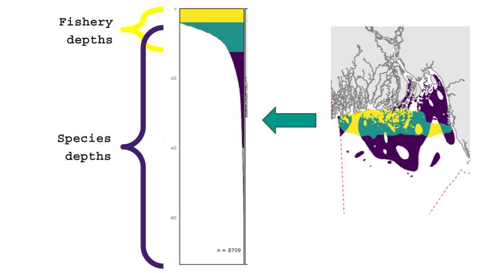
Bangladesh artisanal fisheries (Haque et al.). On a 2D map, the knifetooth sawfish range and the artisanal fishery overlap across much of the Bangladesh shelf. In 3D the story changes: the fishery works the shallow band near the surface, while much of the sawfish range sits deeper, giving the species a partial depth refuge. I reproduce this analysis with rasterize_ranges() and calc_volume_overlap().

Abiotic habitat across the full 3D range (Aitchison et al., VanderWright et al.). A species does not experience the ocean at the surface alone. It lives across a range of depths, each with its own temperature and oxygen. I characterise the conditions a species actually experiences across its full depth range, which can look very different from surface values alone. My example workflow runs this for 1,213 chondrichthyan species, using woa_load_nc() and extract_rast_volume().

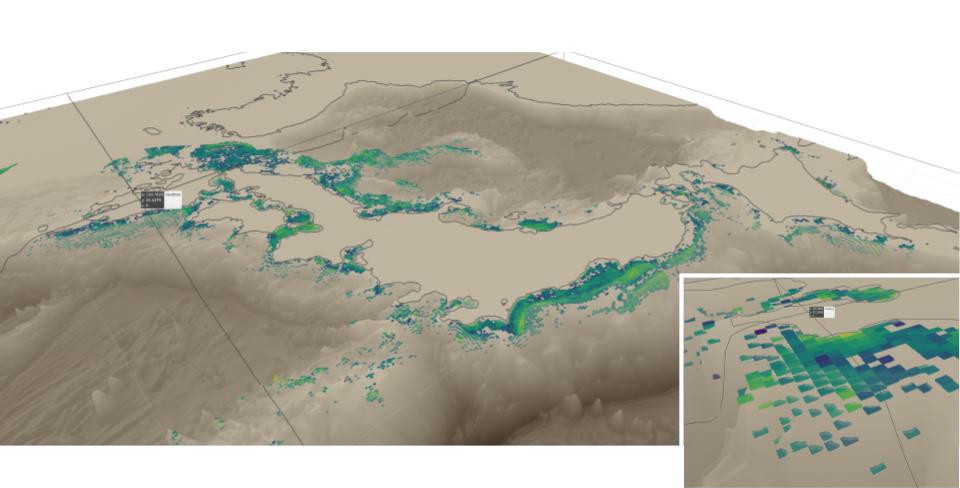
Depth-aware fishing effort. Bottom-contact gear does its work on the seafloor, not at the surface, so a flat 2D heatmap puts the pressure in the wrong place. I drape benthic fishing effort onto the seafloor instead, showing where that gear actually concentrates. The example uses Global Fishing Watch data over the Japan EEZ.

Building it like software

My approach was to treat research code as software, which was also a theme of my Sharks International talk. I built the package to be open source, version-controlled with Git, written in a functional style with small composable functions, and covered by an automated test suite. My aim was reproducibility: another researcher should be able to install the package, follow a documented vignette, and rerun the analysis on their own species or region.

I chose an R package structure to make the analysis reusable and to document how each function works. Scattered scripts are hard to reuse, so packaging the methods removes that friction. When reuse gets easier, I get more analysis done with less rework. The package structure also lets me write tests that confirm the functions behave as expected, so I can verify the methods rather than just trust them.

Open source is the other half of the idea. It lets me share the work with other researchers, who can in turn contribute their own findings and use cases and make the package more useful over time. It keeps the barrier to entry low, so anyone can pick it up and use it. The hope is that good methods can travel beyond a single lab and help folks working on these questions across the world.

This foundation is also what lets me use AI well. AI can generate a large amount of code quickly, but only a tested, version-controlled, well-structured project gives it a clear map to follow and gives me a fast way to check its work. The test suite is what makes this safe: it tells me right away if a change, whether mine or AI-assisted, breaks something that used to work. So I can move quickly without losing confidence that the methods still do what they should.

Status and future directions

sharkabc3d is in active development, with the core in place and proven. The priority functions for volume calculation, environmental extraction, World Ocean Atlas handling, and plotting are implemented, documented with roxygen2, and tested. I presented the package at Sharks International 2026 in Sri Lanka, where it carried three separate analyses. Next, I am writing the worked vignettes that recreate the past lab analyses end to end.

Planned expansions of features:

3D species distribution models that extend traditional 2D SDMs by incorporating depth as an explicit dimension.
Incorporating shark tagging data for direct, observed depth use.
Spatial protection and management analysis, including 3D overlap with marine protected areas.
Support for Copernicus Marine data alongside World Ocean Atlas.
Longer term, a space-time cube model combining raster and vector data into a unified space-depth-time structure.

Next steps:

Increase awareness of the package and number of users by publishing journal article describing the package and its functionality
Create collaborator guides to foster open-source contributions
Keep using this package and refining it as I use it for my own work.

Reflection

The most satisfying part of this work has been the consolidation. A lot of good conservation analysis lives only inside the manuscript it was built for, as scripts that are hard to find and harder to rerun. Turning that into a package that the next person can install and reuse feels like the right way to make methods last beyond a single paper.

There is so much work that goes into figuring out the details, like troubleshooting, updating packages, and testing functions. When we write one-off scripts, they end up as a static snapshot in time. Not just of the code itself, but also with the accompanying versions of R, other packages, operating systems, the data. With so many variables, there is no guarantee that these static scripts will run successfully in the future. If every scientist had to do all of this work each time, it would be a massive time sink and duplicated effort across projects.

By bundling my code into a package, I can work through these details and solve problems for everyone working with these tools at the same time. I find it very rewarding to be able to scale my collaborator’s efforts and increase their ability to do science. In this role, I also get to understand many projects, each with different authors, approaches, and specific topics. By developing this package to apply to a range of scenarios, it forces me to think about the fundamental patterns of thinking across the problem space. I find myself greatly enjoying this process!

I have experience working across a range of disciplines, from ecological research, UX/UI in immersive reality, and freelance software development. In all of these situations, I showed up with almost no infrastructure or support for software. Even when starting out, I was often the only person working on these projects with any software knowledge. No designers, no project managers, of course no other software developers. No one to turn to for help with technical challenges. I solved problems on my own, constantly. I think this taught me the grit and confidence I carry into my work now.

Skills demonstrated

R package development (terra, sf, roxygen2, testthat)
3D and 2.5D marine spatial analysis
Geospatial data engineering and raster algebra
Working with scientific data APIs (IUCN Red List, Global Fishing Watch)
Oceanographic and bathymetric datasets (World Ocean Atlas 2023, GEBCO)
Reproducible research and functional programming
Git version control and automated testing
Effective and responsible AI integration into scientific software development
Data visualisation for spatial and depth-stratified data
Scientific communication (conference presentation, documentation)